Forecasting Energy Markets
Introduction
Over the past several years, global events have rocked the energy markets: the Covid-19 pandemic caused the price of oil to crash, while a combination of inflation and the sanctions placed on Russia due to its invasion of Ukraine have caused the price of oil and natural gas to skyrocket. As a result, it is important to be able to forecast energy markets accurately despite global uncertainty on a day-to-day basis.
With this in mind, my project aims at developing a tool that can forecast energy markets one period into the future consistently and accurately and in a time-effective manner. This tool can help local governments allocate resources in times of volatility and help investors and high-frequency traders optimize trading futures. Specifically, by pulling publicly available data, I will train different univariate models on past values to forecast next day values.
Tools
I will be creating these models using Python. In particular, I will be using the pandas and numpy libraries to clean the data, the requests and json libraries to pull and parse the data, and the sklearn library to prepare the data. I will be using a XGBoost regressor, a Support Vector regressor, and a Random Forest regressor to forecast the data.
import requests
import pandas as pd
import numpy as np
import json
import matplotlib.pyplot as plt
import itertools
import math
import datetime

import xgboost as xgb
from xgboost import XGBRegressor
from sklearn.ensemble import RandomForestRegressor
from sklearn.svm import SVR

import sklearn
from sklearn.metrics import mean_squared_error
from sklearn.model_selection import GridSearchCV
from sklearn.model_selection import cross_val_score
from sklearn.model_selection import train_test_split
from sklearn.metrics import mean_absolute_error
from pylab import rcParams
rcParams['figure.facecolor'] = 'white'
rcParams['axes.facecolor'] = 'white'
rcParams['figure.figsize'] = 12,6
Pulling Data from the U.S. Energy Information Administration
The U.S. Energy Information Administration (EIA) collects and disseminates energy data to the public to promote efficient markets, sound policy making, and public education. The EIA makes its data available through dashboards available here: https://www.eia.gov/tools/. For people who want to pull data locally, the EIA provides documentation for their API here: https://www.eia.gov/opendata/documentation.php. To pull the data, one needs to register an API key. I blurred mine out, but one can easily be obtained from their website. However, their API has several problems. The first is that when trying to determine which data to pull, the options are often hidden, making querying data tedious. Additionally, the maximum number of points that can be pulled per request is 5000 datapoints. If one wants to pull more data, they would either have to paginate or or filter their data in the API call, as opposed to in a dataframe tool, like Pandas, which would be typically more well known by the user. My first class, LoadQuery, addresses these issues.
The class LoadQuery begins by looping through the different pages available, from which the user can select which data they want while having all options available, and then choose which dataset they want to pull. Next, the user will choose the periodicity of the data, if it comes in multiple formats, as well as the type of data that they want to pull, again, if the data comes in mulitple formats. Once chosen, the program will then paginate through the queries until all data is pulled. The data is then turned into a Pandas dataframe format, which can be accessed through the .df attribute of the LoadQuery object. The dataframe will be indexed by date.
date_switch = {'annual':'%Y',
                   'monthly':'%Y-%m',
                   'daily':'%Y-%m-%d'}

class LoadQuery:
    def __init__(self, header = "",page = "", key = "",data = None, frequency = None,response = None, df = None, format = None):
        self.header = 'https://api.eia.gov/v2'
        self.page = page ##Which page you want to access. Created by running load_page
        self.key= #XXXXXXXXX
        self.data = data ##The data you want to access with the query. Created by running choose_query
        self.frequency = frequency
        self.response = response
        self.df = df
        self.format = format

    def load_page(self):
        ##When running load_page, this creates
        api_url = self.header+self.page+self.key
        response = requests.get(api_url)#, verify = False)
        response = response.json()
        if 'frequency' not in response['response'].keys():
            print('Choose your id')
            check = []
            for i in response['response']['routes']:
                print("id: ", i['id'], " Name: ", i['name'],'\r')
                check.append(i['id'])
            next_page = input()
            if next_page not in check:
                print('What you typed was not an option')
                self.load_page()
            else:
                self.page+='/'+next_page
                self.load_page()
        api_url = self.header+self.page+self.key
        response = requests.get(api_url)
        self.response = response.json()


    def choose_frequency(self):
        if len(self.response['response']['frequency']) == 1:
            self.frequency = self.response['response']['frequency'][0]['id']
        else:
            print('Choose the frequency')
            check = []
            for i in self.response['response']['frequency']:
                check.append(i['id'])
                print(i['id'])
            frequency = input()
            if frequency in check:
                self.frequency = frequency
            else:
                print('What you typed was not an option')
                self.choose_frequency()

    def choose_data(self):
        if len(self.response['response']['data'].keys()) == 1:
            self.data = list(self.response['response']['data'].keys())[0]
        else:
            print('Choose the data type')
            check = []
            for i in self.response['response']['data'].keys():
                check.append(i)
                print(i)
            data = input()
            if data in check:
                self.data = data
            else:
                print('What you typed was not an option')
                self.choose_data()

    def create_info(self):
        api_url = self.header+self.page+self.key+'&data[]='+self.data+'&frequency='+self.frequency
        response = requests.get(api_url)
        self.response = response.json()

    def create_every_response(self):
        self.format = date_switch[self.frequency]
        api_url = self.header+self.page+"/data"+self.key+'&data[]='+self.data+'&frequency='+self.frequency
        response = requests.get(api_url)
        data = response.json()
        final = data['response']['data']
        total = data['response']['total']
        offset = 5000
        if total <= 5000:
            self.response = final
        else:
            num_loops = math.floor(total/5000)
            offset = 5000
            for i in range(0,num_loops):
                api_url = self.header+self.page+"/data"+self.key+'&data[]='+self.data+'&frequency='+self.frequency+'&offset='+str(offset)
                response = requests.get(api_url)
                data = response.json()
                final += data['response']['data']
                offset += 5000
                percent = (offset-5000)/total*100
                print("%.2f"%percent,'% of the way done')
            self.response = final

    def get_total_number_of_data_points(self):
        api_url = self.header+self.page+"/data"+self.key+'&data[]='+self.data+'&frequency='+self.frequency
        response = requests.get(api_url)
        response = response.json()
        return response['response']['total']

    def create_df(self):
        api_url = self.header+self.page+"/data"+self.key+'&data[]='+self.data+'&frequency='+self.frequency
        response = requests.get(api_url)
        data = response.json()
        self.df = pd.DataFrame(data['response']['data'])

    def return_url(self):
        url = self.header+self.page+"/data"+self.key+'&data[]='+self.data+'&frequency='+self.frequency
        return url

    def create_data_df(self):
        self.df = pd.DataFrame(self.response)

    def create_index(self):
        self.df['period'] = pd.to_datetime(self.df['period'],format = self.format)
        self.df['time_idx'] = pd.DatetimeIndex(self.df['period'])
        self.df = self.df.set_index('time_idx')
        self.df = self.df.sort_values('time_idx')

    def run_all(self):
        self.load_page()
        self.choose_frequency()
        self.choose_data()
        self.create_info()
        self.create_every_response()
        self.df = pd.DataFrame(self.response).drop_duplicates()
        self.create_index()
        print('Data has been obtained')
Building the Models
To build and determine the best model, I built the ForecastModel class below. A ForecastModel object takes four parameters: the data one wants to forecast which was pulled from the query, the number of past periods to train the models on, the number of periods to forecast, and the name of the column in the dataframe being passed that contains the data.
I perform a GridSearch across a Support Vector regressor, a XGBoost regressor, and a RandomForest regressor. First, I
To build the models, I first call the shift_values() method to shift the values being predicted up a row so that the features in each row will forecast the value for the next day. Next, I call train_models(), which calls the models and performs a GridSearch, trains each model on a 80/20 split, and then performs a forecast by using the datapoints forecasted as the features. I then store the error and the predictions for each model. Afterwards, I align the predictions with the dates they correspond to through update_df().
Finally, I call plot_best_model() to plot with the smallest MAE, while plot_data() plots all three models trained from the GridSearch. Calling find_best_model() works through the above steps and plots the best model. Calling the regressors attribute will display the final models created for each regressor. Below, I work through two examples.
params = {
'Support Vector Regressor':{"C": [0.5, 0.7], 'kernel':['rbf', 'poly']},
'RandomForest':{'max_features':[1.0,'sqrt'],'min_samples_split':[2,5,10],'min_samples_leaf':[1,2,4],'bootstrap':[True,False]},
'XGBoost':{'min_child_weight': [5, 7, 9],'colsample_bytree': [0.2, 0.4, 0.6],'max_depth': [5, 7, 9]}
}

class ForecastModel:
    def __init__(self, df=None, num_shifts = None, num_predict = None, col = None,
                 error = None, test=None, predictions = None, final_df = None, final_date = None, first_date = None, regressors=None):
        self.df = df
        self.col = col
        self.num_shifts = num_shifts
        self.num_predict = num_predict
        self.data = self.shift_values()
        self.error = error
        self.test = test
        self.predictions = predictions
        self.final_df = final_df
        self.final_date = final_date
        self.first_date = first_date
        self.regressors = regressors

    def create_regressors(self):
        regressors = {
            'Support Vector Regressor': [SVR()],
            'RandomForest':[RandomForestRegressor()],
            'XGBoost': [XGBRegressor()]
        }
        self.regressors = regressors

    def shift_values(self):
        df_dummy = self.df[[self.col]].copy()
        for i in range(1,self.num_shifts+1):
            name = self.col + "_shift " + str(i)
            df_dummy[name] = df_dummy[self.col].shift(i)
        df_dummy[self.col] = df_dummy[self.col].shift(-1)
        df_dummy = df_dummy.dropna(how='any',axis=0)
        y = df_dummy[self.col]
        X = df_dummy.drop(self.col,axis=1)
        return X,y

    def train_models(self):
        X,y = self.shift_values()
        X_train, X_test, y_train, y_test = train_test_split(X, y, test_size=0.2, shuffle=False)
        X_train = np.array(X_train)
        X_test = np.array(X_test)
        y_train = np.array(y_train)
        y_test = np.array(y_test)
        X_pred = X_test.copy()
        self.create_regressors()
        for reg in self.regressors:
            print('Training '+reg)
            model = self.regressors[reg][0]
            #model.fit(X_train, y_train)
            grid = GridSearchCV(model, params[reg])
            grid.fit(X_train, y_train)
            model = grid.best_estimator_
            self.regressors[reg][0] = model
            for i in range(0,len(X_pred)-1):
                new = model.predict([X_pred[i]])
                if i == 0:
                    predictions = np.array([new[0]])
                else:
                    predictions = np.append(predictions,np.array([new[0]]))
                X_pred[i+1] = np.concatenate([new,X_test[i+1][:-1]])
            error = mean_absolute_error(y_test[:-1], predictions)
            self.regressors[reg].append(error)
            self.regressors[reg].append(predictions)
            print(reg+' trained')
        self.test = y_test

    def update_df(self):
        first_date = None
        final_date = None
        length = len(self.df[self.df[self.col] == self.test[0]].index)
        for i in range(0,length):
            x = self.df.index.get_loc(self.df[self.df[self.col] == self.test[0]].index[i])
            new = x + len(self.test) - 1
            if self.df.iloc[new]['value'] == self.test[-1]:
                first_date = x
                final_date = new + 1
                break
        self.first_date = first_date
        self.final_date = final_date
        self.final_df = self.df.iloc[first_date:final_date][[self.col]].copy()[:-1]
        self.final_df['test'] = self.test[:-1]
        for reg in self.regressors:
            self.final_df[reg+' preds'] = self.regressors[reg][2]


    def plot_best_model(self):
        left = 500
        right = 100
        min_error = self.regressors['Support Vector Regressor'][1]
        best_model_name = 'Support Vector Regressor'
        for reg in self.regressors:
            if self.regressors[reg][1] < min_error:
                min_error = self.regressors[reg][1]
                best_model_name = reg

        rcParams['figure.figsize'] = 20,10
        plt.plot(self.df[self.col], label = 'Full Dataset', color = 'black')
        plt.plot(self.final_df[best_model_name+' preds'], label = best_model_name+' Predictions', color = 'blue')
        corr = str(round(self.final_df.corr()[best_model_name+' preds']['value'],3))
        min_error_name = ' MAE: %.3f' % min_error
        plt.title(best_model_name+' Predictions r^2: '+corr+min_error_name)
        plt.legend()
        plt.show()

        plt.plot(self.df[self.col][self.first_date - left:self.final_date + right], label = 'Previous', color = 'black')
        plt.plot(self.final_df[best_model_name+' preds'], label = best_model_name+' Predictions', color = 'blue')
        corr = str(round(self.final_df.corr()[reg+' preds']['value'],3))
        plt.title(best_model_name+' Predictions r^2: '+corr+min_error_name)
        plt.legend()
        plt.show()

    def find_best_model(self):
        self.train_models()
        self.update_df()
        self.plot_best_model()

    def plot_data(self):
        left = 500
        right = 100

        for reg in self.regressors:
            min_error = ' MAE: %.3f' % self.regressors[reg][1]
            rcParams['figure.figsize'] = 20,10
            plt.plot(self.df[self.col][self.first_date - left:self.final_date + right], label = 'Previous', color = 'black')
            plt.plot(self.final_df[reg+' preds'], label = reg+' Predictions', color = 'blue')
            corr = str(round(self.final_df.corr()[reg+' preds']['value'],3))
            plt.title(reg+' Predictions r^2: '+corr+min_error)
            plt.legend()
            plt.show()
Forecasting Natural Gas Futures
Below, I walk through the process outlined above to forecast natural gas futures. Specifically, I will be forecasting the Contract 1 futures prices. Because natural gas contracts expire three business days prior to the first calendar day of the delivery month, Contract 1 contains the calendar month following the trade date. Information can be found at this link: https://www.eia.gov/dnav/ng/TblDefs/ng_pri_fut_tbldef2.asp.
Below, I create a LoadQuery object to pull the data that I want to forecast.
natural_gas_query = LoadQuery()
natural_gas_query.run_all()
Choose your id
id:  coal  Name:  Coal
id:  crude-oil-imports  Name:  Crude Oil Imports
id:  electricity  Name:  Electricity
id:  international  Name:  International
id:  natural-gas  Name:  Natural Gas
id:  nuclear-outages  Name:  Nuclear Outages
id:  petroleum  Name:  Petroleum
id:  seds  Name:  State Energy Data System (SEDS)
id:  steo  Name:  Short Term Energy Outlook
id:  densified-biomass  Name:  Densified Biomass
id:  total-energy  Name:  Total Energy
id:  aeo  Name:  Annual Energy Outlook
id:  ieo  Name:  International Energy Outlook
id:  co2-emissions  Name:  State CO2 Emissions
natural-gas
Choose your id
id:  sum  Name:  Summary
id:  pri  Name:  Prices
id:  enr  Name:  Exploration and Reserves
id:  prod  Name:  Production
id:  move  Name:  Imports and Exports/Pipelines
id:  stor  Name:  Storage
id:  cons  Name:  Consumption / End Use
pri
Choose your id
id:  sum  Name:  Natural Gas Prices
id:  fut  Name:  Natural Gas Spot and Futures Prices (NYMEX)
id:  rescom  Name:  Average Price of Natural Gas Delivered to Residential and Commercial Consumers by Local Distribution and Marketers in Selected States
fut
Choose the frequency
weekly
monthly
daily
annual
daily
11.82 % of the way done
23.64 % of the way done
35.46 % of the way done
47.28 % of the way done
59.10 % of the way done
70.92 % of the way done
82.74 % of the way done
94.56 % of the way done
Data has been obtained
Now that the data has been obtained, I call the dataframe to see the different features and how to filter for Contract 1.
natural_gas_query.df['series-description'].unique()
array(['Natural Gas Futures Contract 4 (Dollars per Million Btu)',
       'Natural Gas Futures Contract 2 (Dollars per Million Btu)',
       'Natural Gas Futures Contract 1 (Dollars per Million Btu)',
       'Natural Gas Futures Contract 3 (Dollars per Million Btu)',
       'Henry Hub Natural Gas Spot Price (Dollars per Million Btu)'],
      dtype=object)
I will filter on the series description ‘Natural Gas Futures Contract 1 (Dollars per Million Btu)’.
series_desc = 'Natural Gas Futures Contract 1 (Dollars per Million Btu)'
natural_gas_data = natural_gas_query.df[(natural_gas_query.df['series-description'] == series_desc)]
natural_gas_data = natural_gas_data.dropna()
natural_gas_data.head()
| time_idx | period | duoarea | area-name | product | product-name | process | process-name | series | series-description | value | units |
|---|---|---|---|---|---|---|---|---|---|---|---|
| 1993-12-20 00:00:00 | 1993-12-20 00:00:00 | Y35NY | NEW YORK CITY | EPG0 | Natural Gas | PE4 | Future Contract 4 | RNGC4 | Natural Gas Futures Contract 4 (Dollars per Million Btu) | 1.894 | $/MMBTU |
| 1993-12-21 00:00:00 | 1993-12-21 00:00:00 | Y35NY | NEW YORK CITY | EPG0 | Natural Gas | PE4 | Future Contract 4 | RNGC4 | Natural Gas Futures Contract 4 (Dollars per Million Btu) | 1.83 | $/MMBTU |
| 1993-12-22 00:00:00 | 1993-12-22 00:00:00 | Y35NY | NEW YORK CITY | EPG0 | Natural Gas | PE4 | Future Contract 4 | RNGC4 | Natural Gas Futures Contract 4 (Dollars per Million Btu) | 1.859 | $/MMBTU |
| 1993-12-23 00:00:00 | 1993-12-23 00:00:00 | Y35NY | NEW YORK CITY | EPG0 | Natural Gas | PE4 | Future Contract 4 | RNGC4 | Natural Gas Futures Contract 4 (Dollars per Million Btu) | 1.895 | $/MMBTU |
| 1993-12-27 00:00:00 | 1993-12-27 00:00:00 | Y35NY | NEW YORK CITY | EPG0 | Natural Gas | PE4 | Future Contract 4 | RNGC4 | Natural Gas Futures Contract 4 (Dollars per Million Btu) | 1.965 | $/MMBTU |
I create the model by passing the dataframe natural_gas_data, train the model by having the previous 50 days predict the next day, forecast the next 150 days, and use the data in the column “value”.
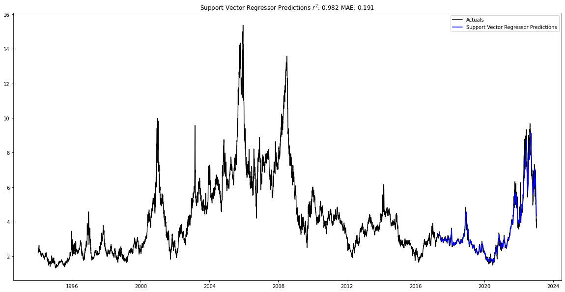
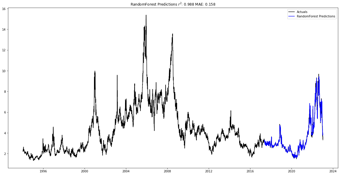
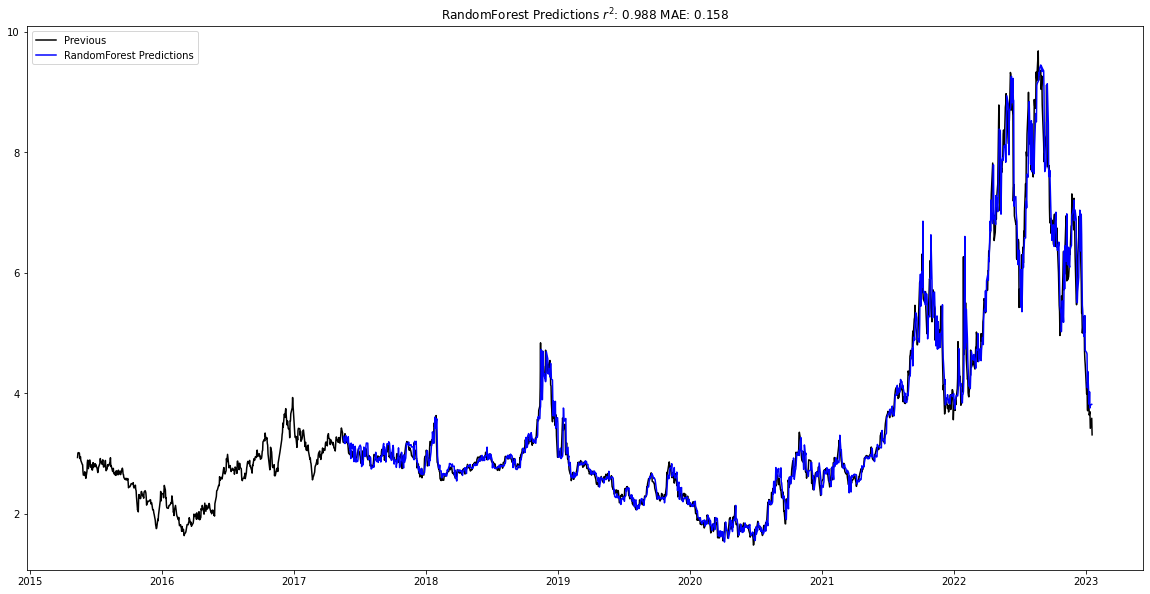
After training the models, the best model is graphed below. The Random Forest regressor was the best model, and had an r2 value of 0.988 with the testing data and a mean average error of 0.158.
natural_gas_forecast = ForecastModel(df = natural_gas_data, num_shifts = 50, num_predict = 150, col = 'value')
natural_gas_forecast.find_best_model()
Training Support Vector Regressor
Support Vector Regressor trained
Training RandomForest
RandomForest trained
Training XGBoost
XGBoost trained
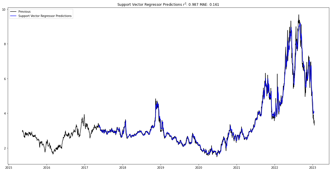
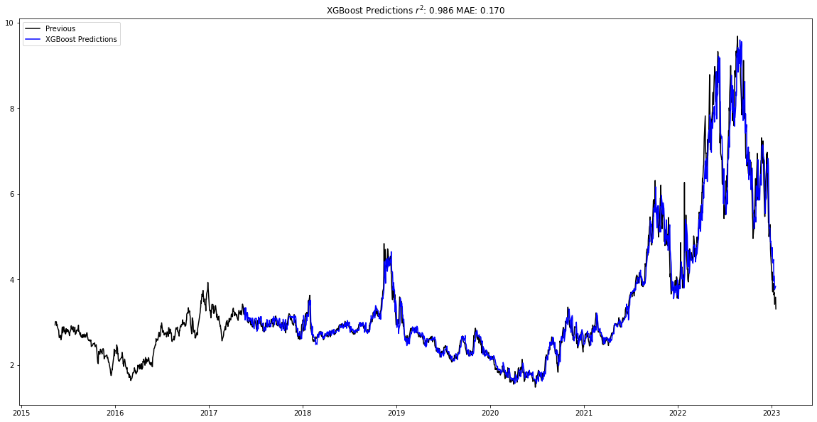
Below I plot the best predictions for each of the different regressors. In addition to the Random Forest regressor, the Support Vector regressor closely predicted the test data, with an r2 of 0.987 and an MAE of 0.161, as well as the XGBoost regression, which had an r2 of 0.986 and an MAE of 0.170.
natural_gas_forecast.plot_data()

Forecasting Petroleum Futures
I’ll now run through the same process by forecasting New York Harbor No. 2 Heating Oil Future Contract 1.
petroleum_forecast = LoadQuery()
petroleum_forecast.run_all()
Choose your id
id:  coal  Name:  Coal
id:  crude-oil-imports  Name:  Crude Oil Imports
id:  electricity  Name:  Electricity
id:  international  Name:  International
id:  natural-gas  Name:  Natural Gas
id:  nuclear-outages  Name:  Nuclear Outages
id:  petroleum  Name:  Petroleum
id:  seds  Name:  State Energy Data System (SEDS)
id:  steo  Name:  Short Term Energy Outlook
id:  densified-biomass  Name:  Densified Biomass
id:  total-energy  Name:  Total Energy
id:  aeo  Name:  Annual Energy Outlook
id:  ieo  Name:  International Energy Outlook
id:  co2-emissions  Name:  State CO2 Emissions
petroleum
Choose your id
id:  sum  Name:  Summary
id:  pri  Name:  Prices
id:  crd  Name:  Crude Reserves and Production
id:  pnp  Name:  Refining and Processing
id:  move  Name:  Imports/Exports and Movements
id:  stoc  Name:  Stocks
id:  cons  Name:  Consumption/Sales
pri
Choose your id
id:  gnd  Name:  Weekly Retail Gasoline and Diesel Prices
id:  spt  Name:  Spot Prices
id:  fut  Name:  NYMEX Futures Prices
id:  wfr  Name:  Weekly Heating Oil and Propane Prices (October - March)
id:  refmg  Name:  Refiner Gasoline Prices by Grade and Sales Type
id:  refmg2  Name:  U.S. Refiner Gasoline Prices by Formulation, Grade, Sales Type
id:  refoth  Name:  Refiner Petroleum Product Prices by Sales Type
id:  allmg  Name:  Gasoline Prices by Formulation, Grade, Sales Type
id:  dist  Name:  No. 2 Distillate Prices by Sales Type
id:  prop  Name:  Propane (Consumer Grade) Prices by Sales Type
id:  resid  Name:  Residual Fuel Oil Prices by Sales Type
id:  dfp1  Name:  Domestic Crude Oil First Purchase Prices by Area
id:  dfp2  Name:  Domestic Crude Oil First Purchase Prices for Selected Crude Streams
id:  dfp3  Name:  Domestic Crude Oil First Purchase Prices by API Gravity
id:  rac2  Name:  Refiner Acquisition Cost of Crude Oil
id:  imc1  Name:  F.O.B. Costs of Imported Crude Oil by Area
id:  imc2  Name:  F.O.B. Costs of Imported Crude Oil for Selected Crude Streams
id:  imc3  Name:  F.O.B. Costs of Imported Crude Oil by API Gravity
id:  land1  Name:  Landed Costs of Imported Crude by Area
id:  land2  Name:  Landed Costs of Imported Crude for Selected Crude Streams
id:  land3  Name:  Landed Costs of Imported Crude by API Gravity
id:  ipct  Name:  Percentages of Total Imported Crude Oil by API Gravity
fut
Choose the frequency
weekly
daily
monthly
annual
daily
3.68 % of the way done
7.36 % of the way done
11.05 % of the way done
14.73 % of the way done
18.41 % of the way done
22.09 % of the way done
25.78 % of the way done
29.46 % of the way done
33.14 % of the way done
36.82 % of the way done
40.50 % of the way done
44.19 % of the way done
47.87 % of the way done
51.55 % of the way done
55.23 % of the way done
58.91 % of the way done
62.60 % of the way done
66.28 % of the way done
69.96 % of the way done
73.64 % of the way done
77.33 % of the way done
81.01 % of the way done
84.69 % of the way done
88.37 % of the way done
92.05 % of the way done
95.74 % of the way done
99.42 % of the way done
Data has been obtained
petroleum_forecast.df.head()
| time_idx | period | duoarea | area-name | product | product-name | process | process-name | series | series-description | value | units |
|---|---|---|---|---|---|---|---|---|---|---|---|
| 1980-01-02 00:00:00 | 1980-01-02 00:00:00 | Y35NY | NEW YORK CITY | EPD2F | No 2 Fuel Oil / Heating Oil | PE1 | Future Contract 1 | EER_EPD2F_PE1_Y35NY_DPG | New York Harbor No. 2 Heating Oil Future Contract 1 (Dollars per Gallon) | 0.821 | $/GAL |
| 1980-01-02 00:00:00 | 1980-01-02 00:00:00 | Y35NY | NEW YORK CITY | EPD2F | No 2 Fuel Oil / Heating Oil | PE3 | Future Contract 3 | EER_EPD2F_PE3_Y35NY_DPG | New York Harbor No. 2 Heating Oil Future Contract 3 (Dollars per Gallon) | 0.89 | $/GAL |
| 1980-01-03 00:00:00 | 1980-01-03 00:00:00 | Y35NY | NEW YORK CITY | EPD2F | No 2 Fuel Oil / Heating Oil | PE1 | Future Contract 1 | EER_EPD2F_PE1_Y35NY_DPG | New York Harbor No. 2 Heating Oil Future Contract 1 (Dollars per Gallon) | 0.827 | $/GAL |
| 1980-01-04 00:00:00 | 1980-01-04 00:00:00 | Y35NY | NEW YORK CITY | EPD2F | No 2 Fuel Oil / Heating Oil | PE3 | Future Contract 3 | EER_EPD2F_PE3_Y35NY_DPG | New York Harbor No. 2 Heating Oil Future Contract 3 (Dollars per Gallon) | 0.88 | $/GAL |
petroleum_forecast.df['series-description'].unique()
array(['New York Harbor No. 2 Heating Oil Future Contract 3 (Dollars per Gallon)',
       'New York Harbor No. 2 Heating Oil Future Contract 1 (Dollars per Gallon)',
       'Cushing, OK Crude Oil Future Contract 3 (Dollars per Barrel)',
       'Cushing, OK Crude Oil Future Contract 1 (Dollars per Barrel)',
       'New York Harbor Regular Gasoline Future Contract 3 (Dollars per Gallon)',
       'New York Harbor Regular Gasoline Future Contract 1 (Dollars per Gallon)',
       'Cushing, OK Crude Oil Future Contract 2 (Dollars per Barrel)',
       'Cushing, OK Crude Oil Future Contract 4 (Dollars per Barrel)',
       'Mont Belvieu, Tx Propane Future Contract 1 (Dollars per Gallon)',
       'Mont Belvieu, Tx Propane Future Contract 4 (Dollars per Gallon)',
       'New York Harbor No. 2 Heating Oil Future Contract 4 (Dollars per Gallon)',
       'New York Harbor Regular Gasoline Future Contract 2 (Dollars per Gallon)',
       'New York Harbor Regular Gasoline Future Contract 4 (Dollars per Gallon)',
       'New York Harbor No. 2 Heating Oil Future Contract 2 (Dollars per Gallon)',
       'Mont Belvieu, Tx Propane Future Contract 2 (Dollars per Gallon)',
       'Mont Belvieu, Tx Propane Future Contract 3 (Dollars per Gallon)',
       'New York Harbor Reformulated RBOB Regular Gasoline Future Contract 2 (Dollars per Gallon)',
       'New York Harbor Reformulated RBOB Regular Gasoline Future Contract 1 (Dollars per Gallon)',
       'New York Harbor Reformulated RBOB Regular Gasoline Future Contract 4 (Dollars per Gallon)',
       'New York Harbor Reformulated RBOB Regular Gasoline Future Contract 3 (Dollars per Gallon)'],
      dtype=object)
petreoleum_forecast_data.df = petroleum_forecast.df[petroleum_forecast.df['series-description'] == 'New York Harbor No. 2 Heating Oil Future Contract 1 (Dollars per Gallon)']
petreoleum_forecast_data.df = petreoleum_forecast_data.df.dropna()
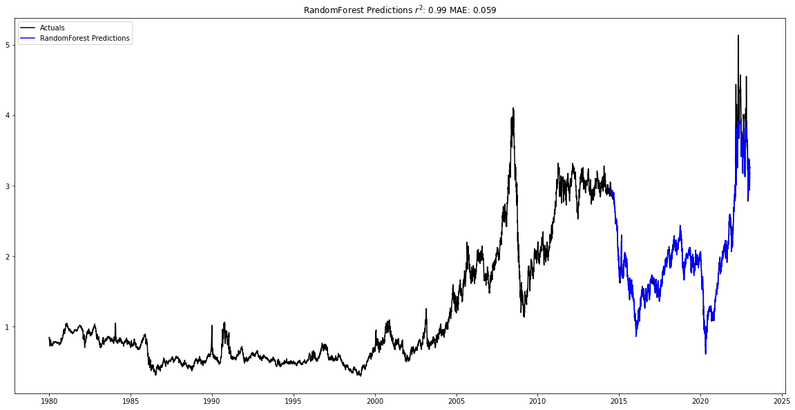
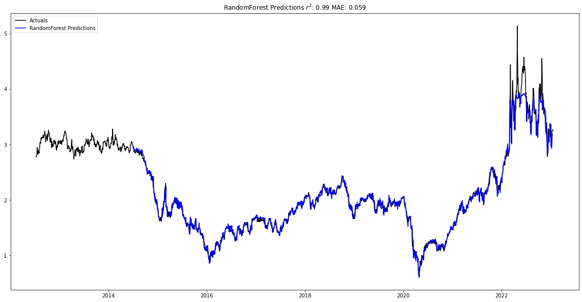
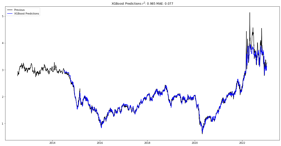
After training the different models, the Random Forest regressor again the smallest MAE at 0.058 and the largest r2 at 0.99 for the testing data.
petroleum_forecast_model = ForecastModel(df = petreoleum_forecast_data.df, num_shifts = 50, num_predict = 150, col = 'value')
petroleum_forecast_model.find_best_model()
Training Support Vector Regressor
Support Vector Regressor trained
Training RandomForest
RandomForest trained
Training XGBoost
XGBoost trained
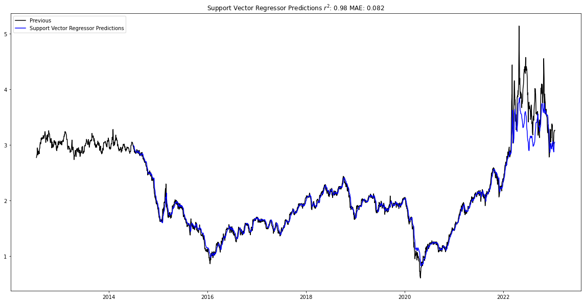
Looking at the other the models, we see that the Support Vector regressor and the XGBoost regressor also captured the trend.
petroleum_forecast_model.plot_data()

Conclusions and Next Steps
Taking a look at the natural gas and petroleum futures predictions, we are able to see that the models captured the volatility due to the Covid-19 pandemic and the invasion of Ukraine in their forecasting fairly well. Although the petroleum forecasts had more difficulty during the invasion of Ukraine, the Random Forest model captured the overall movement. To address this, a model that includes news events could be helpful, as I discuss below. As a result, it seems that univariate time-series models can be useful and cost-effective in forecasting markets in the short term.
I believe that there are several ways to improve this project. First, when testing the models across other datasets, some models were more seasonal than the data shown above. As a result, when data appears more seasonal, performing a seasonality decomposition could increase model performance while decreasing complexity. Secondly, there were some datasets where models had more difficulty making predictions. Creating a multivariate model that incorporates features such as GDP, local and international conflicts, different weather events, and location could improve model performance as well. Finally, this model only included 1 period forecasts. It would be interesting to see how this approach fares in predicting multi-period forecasts, such as a 7 day forecast or a 30 day forecast. To accomplish this, including an RNN neural net model could be helpful in creating these forecasts.
